The Flaw of Averages: Sequence of Returns Risk and Volatility Drag in Retirement

November 23, 2025

Even if your portfolio earns 6% per year on average, you can still run out of money in retirement. That’s because retirees face sequence of returns risk and volatility drag: the order and variability of returns sometimes matter more than your long-run averages. This article explains why relying on deterministic ‘average return’ models can be dangerous when you are close to your retirement, and how these risks derail your plan.

Introduction

For much of the last century and into the 21st, US and UK equities have delivered real returns of around 6.6% and 5.4% per year^[1] respectively, implying a risk premium of roughly 4-6 percentage points over short-term government bills. These constants have become the bedrock of modern private financial planning: calculate the monthly savings, define an asset allocation, look at the historical asset return and specify a future expected return, and let the compound return determine the future asset value.

For the accumulators in the workforce, this reliance on averages is largely forgivable. Over a multi-decade horizon, the law of large numbers tends to smooth out the market volatility, allowing patient accumulators to eventually capture the mean.

However, once the investor transitions to the decumulation phase, this becomes a dangerous simplified assumption.

For recent retirees, or those approaching their target date, the average return becomes secondary concern; the chronology and volatility of those returns become paramount.

This is the domain of Sequence of Returns Risk and Volatility Drag.

The Tyranny of Timing

Consider two hypothetical retirees at age 60, Alice and Bob. Both concluded their professional lives on Friday at the office. The atmosphere is one of victorious relief — customary toasts, warm speeches about “new chapters”, and the clinking of glasses to celebrate the once-in-a-lifetime occasion.

As they walk out the door, their futures look indistinguishable. They each possessed a nest egg of $1,000,000, with inflation-adjusted expense of $40,000 per year. According to the glossy financial projections tucked inside their briefcase, they are destined to make an real average return (after inflation) of exactly 3% over the next 25 years. They have “made it”.

However, we will introduce a twist to this story: the chronology of the returns.

• Alice happens to retire into a roaring bull market. In her first three years, her investment returns are 30%, 20%, and 10%. Only then does she face a slump of -30% and -15%, before market reverts to run of unremarkable “normal” returns.
• Bob faces the opposite fate, He retires into recession, suffering negative returns in the first two years (-30%, -15%), followed by large bull market (30%, 20%, 10%), and thereafter same normal returns as Alice. They both experience the same return, just at different order.

Let’s observe what happens when we apply these returns to their identical starting positions and withdrawal pattern:

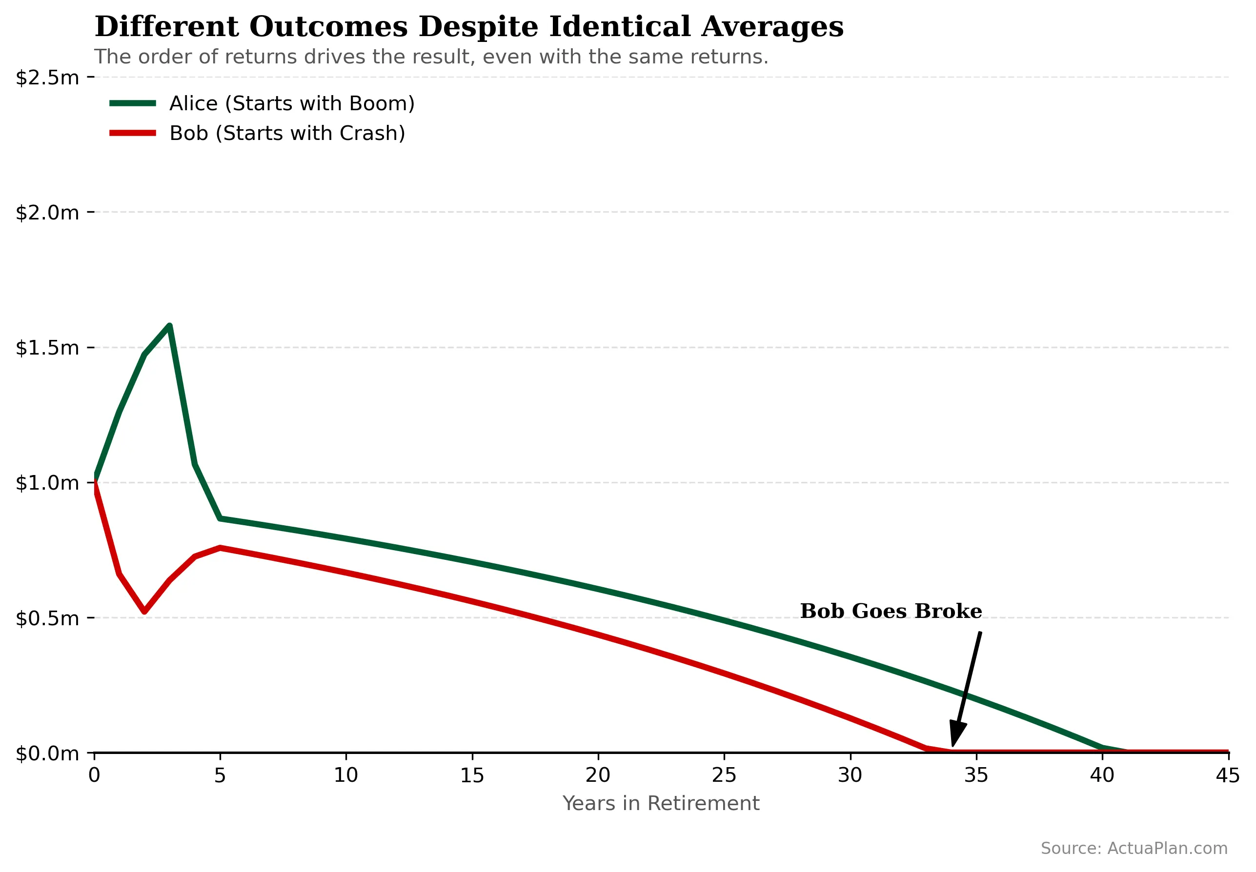
We can see that even with the same return in the first 5 years but with order reversed, they have different portfolio values at year 5:

• Alice: $865,624
• Bob: $757,236

After only 5 years, Alice is roughly 14% better off than Bob, despite facing the same set of returns. From that point onward, if both simply earn a steady 3% real return, Bob’s portfolio runs dry in year 34 (age 94). Alice’s lasts until year 41 (age 101) – hardly guaranteed, but reasonable satisfactory by the standards of retirement planning.

Now, what if we repeat the business cycles over the whole projections?

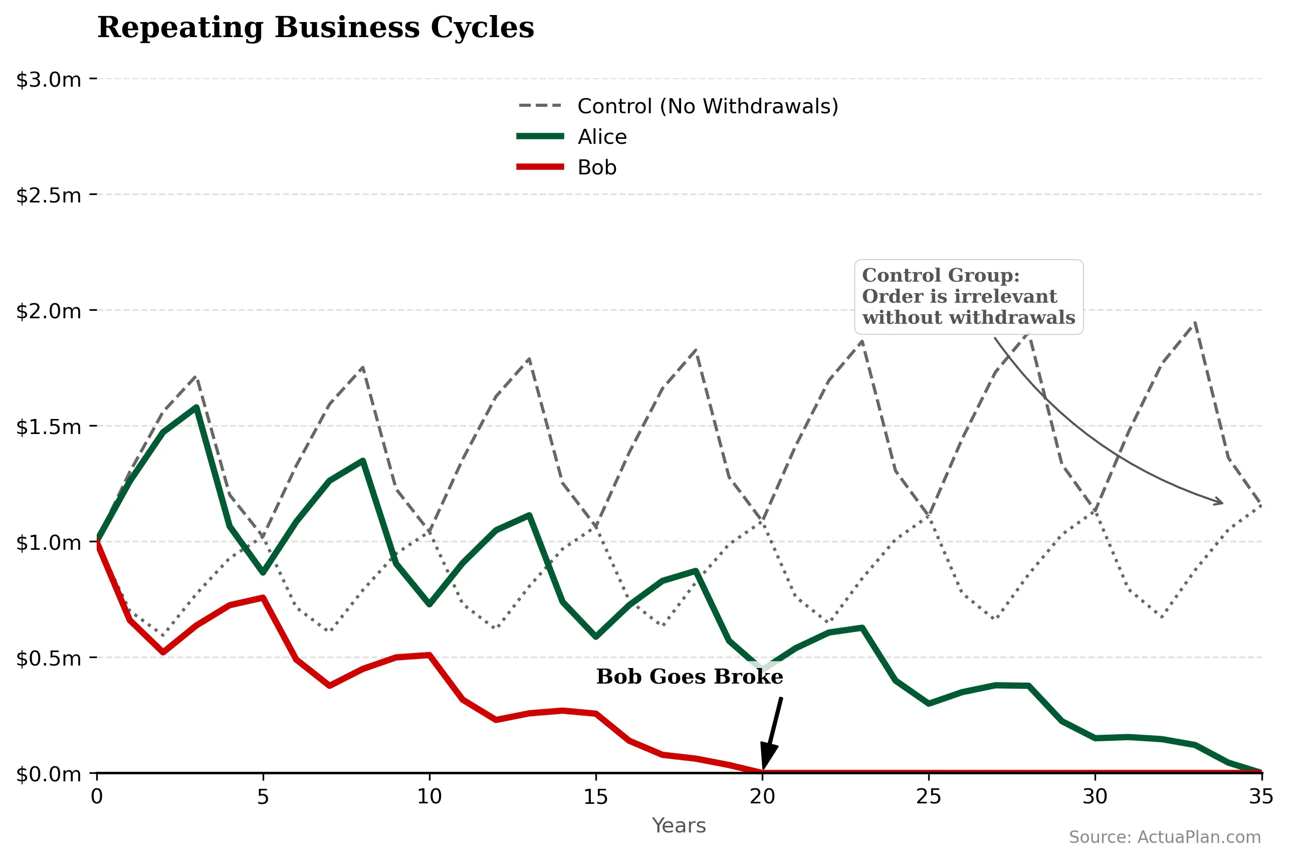
The disparity is now staggering. Bob’s portfolio is exhausted around year 20, at age 80 – years earlier than he expected. Alice, by contrast, still has funds well into her nineties (year 30+).

The Mechanism of Destruction

The phenomenon destroying Bob’s retirement has a name: Reverse Dollar-Cost Averaging. When markets decline early in retirement, fixed withdrawals represent an ever-larger percentage of remaining portfolio. These high withdrawal percentages lock in losses and leave less capital behind to benefit from the recovery when it eventually comes, causing irreversible damage.

For Alice, she was fortunate to experience boom in the first 3 years, which means that she will have higher portfolio value at the start with lower effective withdrawal rate (as the fixed $40,000 per year is smaller percentage of portfolio value compared to Bob).

Yet even Alice is not entirely safe. You may have noticed that her plan, which initially seemed to last until year 41, now runs dry closer to year 35 once we introduce repeated business cycles. Another mathematical assassin is at work.

The Hidden Assassin: Volatility Drag

Let’s focus on the crash sequences we introduced in this post. A quick careless mental arithmetic shows that the crash sequence of [-30%, -15%, 30%, 20%, 10%] do, in fact, add up to the average return of 3% per year:

Arithmetic mean = (- 0.3 – 0.15 + 0.3 + 0.2 + 0.1)/5 = 0.03 = 3%

On the surface of it, it looks reassuring. The “average” return matches the neat 3% in the brochure. But what if you compound the $1 over the crash sequences?

$1 * (1 – 0.3) * ( 1-0.15) * (1 + 0.3) *(1 + 0.2) * (1+ 0.1) ≈ $1.02

In other words, after 5 years you have only about 2% more than what you started with. Spread that over 5 years you get a geometric return of roughly 0.4% per year – a far cry from the 3% suggested by the arithmetic mean.

The gap between the two is volatility drag. When there is volatility in the returns, the geometric return falls below the simple average. The gap widens as volatility increases.

Fortunately, most large institutions do understand the distinction and will often quote long-run geometric returns in their projections. That is helpful, but it does not make the problem disappear. It simply means expected volatility drag has already been baked into the number. Still, larger than expected volatility will reduce the expected return.

What should investors do with this?

For an individual saver or retiree, a few practical rules follow:

• Ask what kind of “average” you are looking at. If a projection is based on arithmetic averages, the headline return is almost certainly optimistic for a volatile portfolio.
• Be wary of “Straight lines”. Even geometric return with volatility drag baked in would not capture the risk when good and bad years arrive, and hence sequence-of-return risks should be stress-tested on your portfolio.

When Crashes Hurt Most

So far we have followed a single 5-year crash sequence through Alice and Bob’s retirement. We can go one step further and ask a broader question: if that same five-year pattern of –30%, –15%, +30%, +20%, +10% were to strike at different points in your life, when would it be most damaging?

The following charts map this out. We simulate an investor who starts saving at 25, retires at 60, and in baseline scenario, earns a steady real return of 3% a year throughout. We then slide the same 5-year crash sequence along this life cycle and quantify the impact to the total withdrawal (spending) and terminal wealth. To isolate the pure-timing effects, we have re-scaled the 5-year market crash sequence so that geometric sequence remain 3% (i.e. no volatility drag):

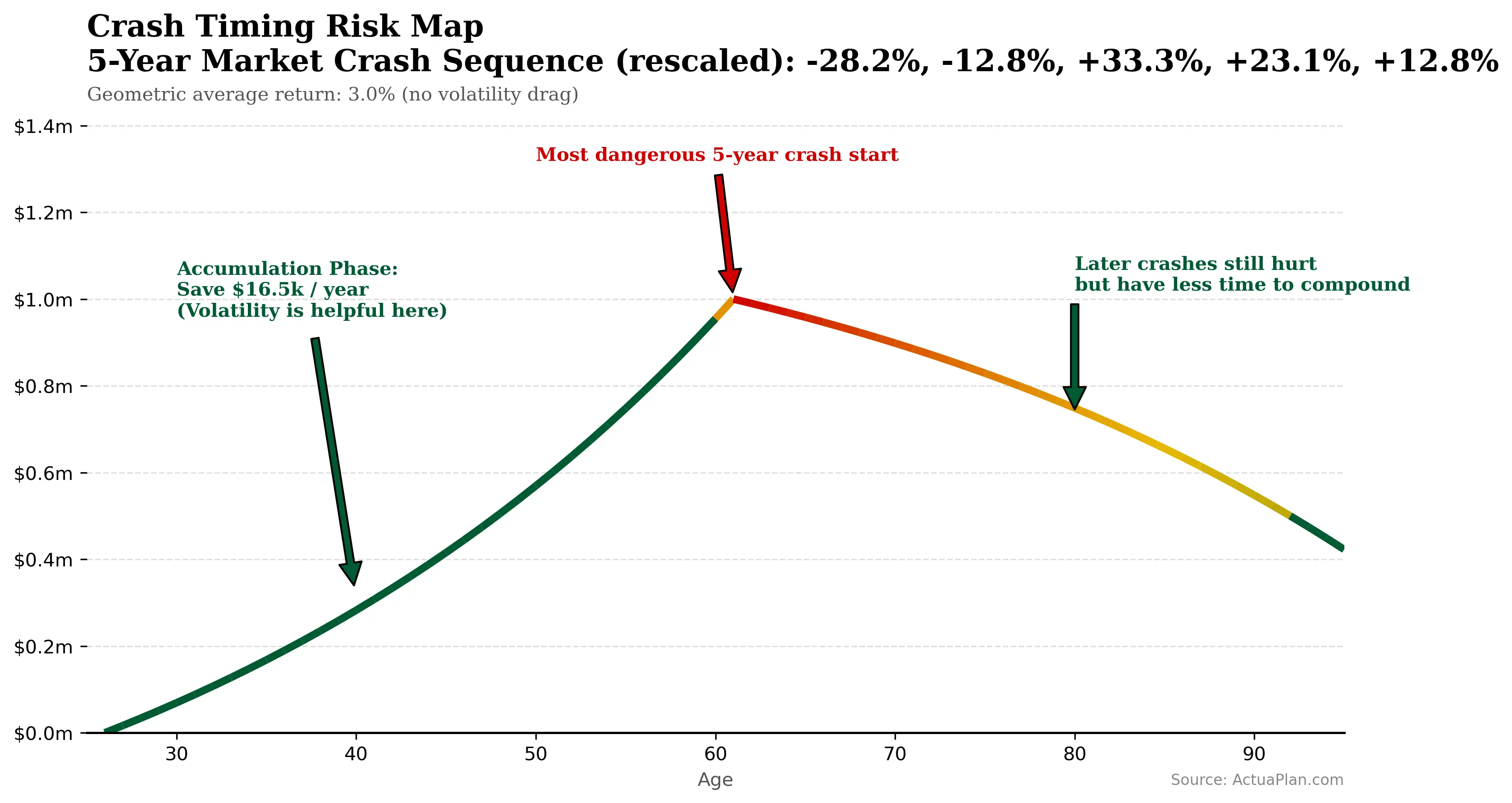
In the first chart, the horizontal axis shows age and the vertical axis shows the portfolio value over time, with the path colored by how severely it is hit. Crashes in the accumulation phase (from the 20s to close to retirement age) are uncomfortable but oddly helpful: you’re saving each year, and the crashes lets you buy more cheaply. Crashes later in life, in your 70s and 80s, still hurt but have less time to compound. The deepest damage appears when the crash starts just before or just after retirement, when the withdrawals begin and the portfolio value is at its peak.

The impact to the total withdrawals and terminal wealth is shown in the next chart, where the coloring of the path is derived.

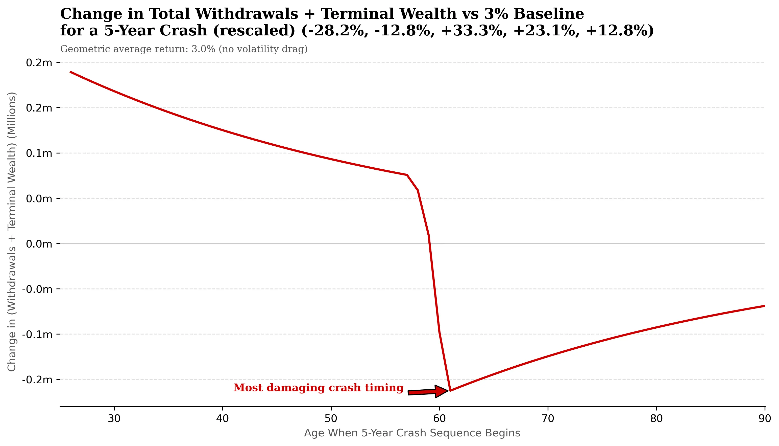
The second version of the charts runs the same experiment, using the original crash sequence where volatility drag is present:

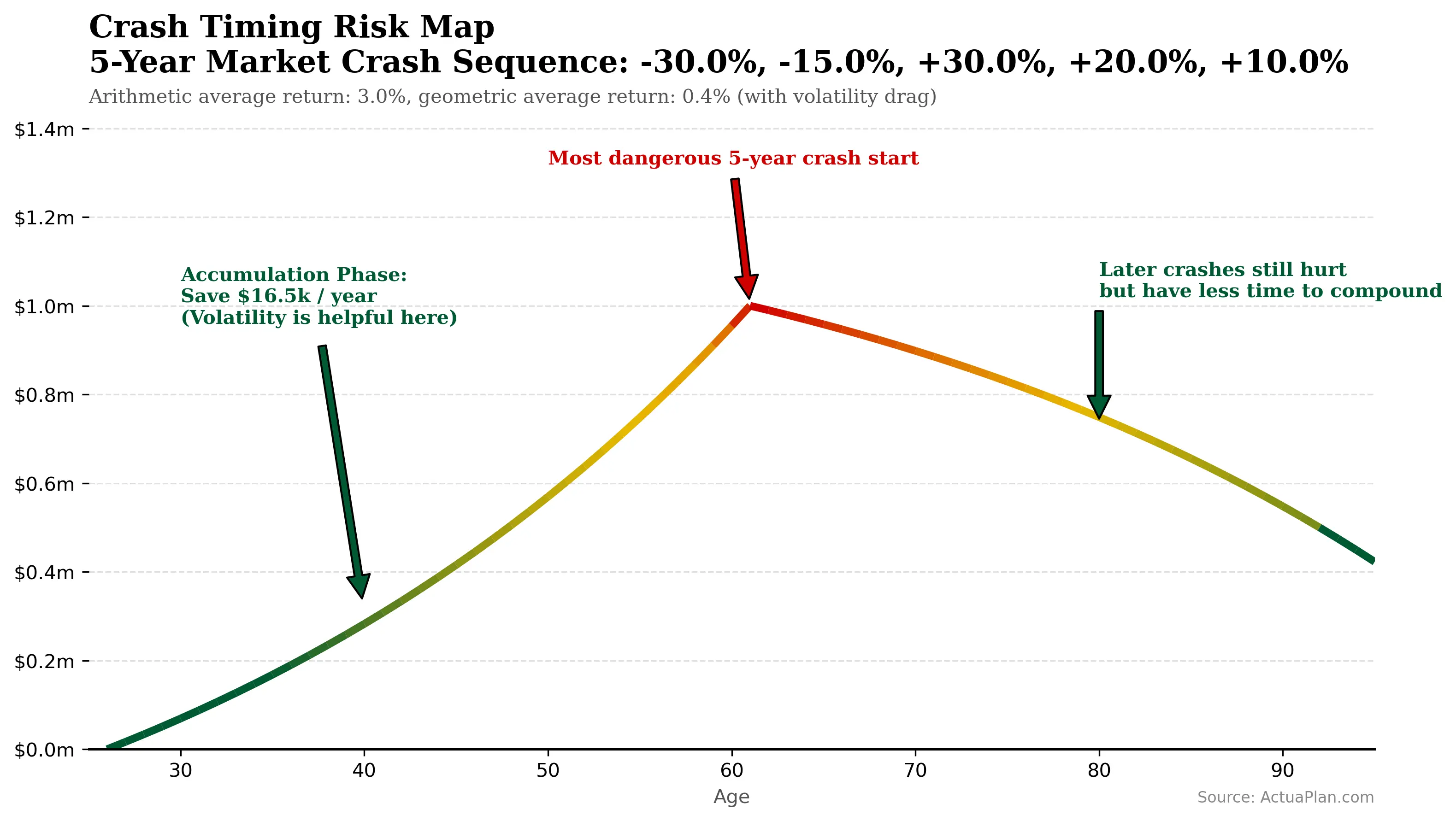
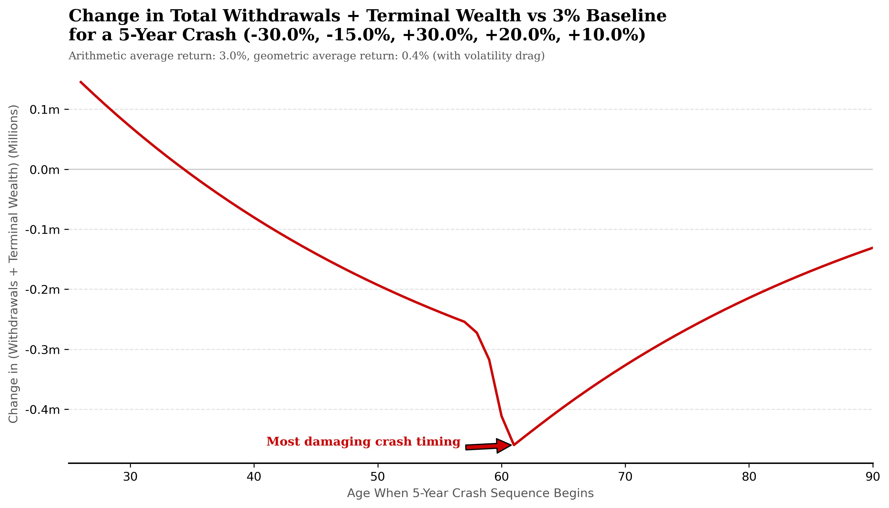
The shape of the curve changes slightly. Notably, the entire impact line has shifted downwards. At almost every age, the investor now ends up worse off than in the smooth 3% world, with more pronounced impact around the retirement age, where the portfolio value is largest.

Taken together, these pictures make the combination of sequence risk and volatility drag uncomfortably clear:

• The Sequence-of-Returns risk is most dangerous in the years just before and after retirement, when withdrawals begin and the portfolio value is at its peak.
• Volatility drag, which lowers the true compounded return, hurts most when it is applied to a large pot of money – again, typically just as someone approaches or enters retirement.

The Villain: The Comfort of Linearity

Yet the tools most people see show none of these complexities. If you have a pension, a unit-linked insurance policy, or a retirement account with large institution, you have almost certainly been shown a table of neat projections – “low”, “median”, “high”. Each column traces a smooth curve into the future and tells a reassuring story: If your money grows at this steady rate, here is what you might have at 65, or 75, or 85.

There is nothing inherently wrong about these numbers. In many cases they are based on reasonable long-term, volatility-adjusted geometric return assumptions. The real problem is what is missing. Those glossy charts quietly assume that markets will deliver the same tidy percentage every year, like interest on a bank deposit. Volatility is edited out of the picture.

But retirees don’t live in those realities. They live through sequences of returns, in which a bad year at a bad time can pose irreparable damage to their retirement funds. Volatility drag means that more bumpy future will leave the retirees with less returns.

The Stochastic Solution

Alice and Bob’s divergent fates, despite identical portfolio and average future returns, expose the fundamental inadequacy of deterministic retirement planning. The answer is not to abandon planning but to embrace uncertainty properly.

ActuaPlan runs thousands of potential market scenarios with realistic volatility via Monte Carlo Simulation. It reveals uncertainty of the distribution of retirement outcomes. Instead of a single “expected” result, you see probabilities: x% of chance of success.

This is where modern retirement planning must go. Not “you will have $2.3million at 95”, but “you have an 85% probability of maintaining your lifestyle throughout the whole lifespan, with targets such as purchasing house, bequests, and with these specific adjustments available if unexpected events happen”.

References

[1] Global Investment Returns Yearbook 2025 | UBS Global

About the author

Roen is a Fellow of the Society of Actuaries (FSA) and a Chartered Enterprise Risk Actuary (CERA) working in life insurance. His work focuses on Solvency II, capital management, and asset–liability management, with deep experience in financial and stochastic modelling. On this site, he uses the same actuarial tools applied in insurers to help individuals think more rigorously about retirement and long-term financial risk.

References

- UBS GlobalGlobal Investment Returns Yearbook 20252025. Retrieved December 2025. https://www.ubs.com/global/en/investment-bank/insights-and-data/2025/global-investment-returns-yearbook-2025.html